ALMA Spectral Imaging Tutorial
Getting started
For this tutorial we will be working with the spectral line data of source ALESS49 from the ALMA Cycle 4 project 2016.1.00754.S. Observations of ALESS49 were taken as part of seven execution blocks (EBs) at ALMA. Each of these EBs when fully calibrated are 15G, so for convenience we've done a few things to make a smaller dataset to work with.
The following has been done to the seven EBs to create the data product you will be working with:
- The calibrated data for ALESS49 has been split out and averaged in time to 13.2s into a separate measurement set (MS), one for each EB.
- Each of these new 'ALESS49'-only MSs have then been concatenated into a single MS.
These steps create a single MS named ALESS49_ALL_EBS.ms which can be downloaded here (total size 3.8GB). The imaging steps we will work with are within the scriptForSpectralImaging.py here.
A publication using these data was published by Wardlow et al. 2018 here
STEPS 0 and 1: CONTINUUM SUBTRACTION and FULL SPECTRAL WINDOW IMAGING
The first thing to consider is the level of continuum emission in the source. To perform accurate science with detected spectral lines we need to work with continuum subtracted data; conversely to do good science with the source continuum emission we need to use only line free channels!
To guage the level of continuum and find the line free channels we need to make data cubes of the each of the science spectral windows. This can be achieved using Step 0 in the script for this session.
STEP 0: Generate full cubes
Before running the script you will need to fill in the following missing values in the script, (using calculation similar to those seen in todays simple continuum imaging tutorial here) :
cell, the size of the pixels in arcsec. This should be a fraction (1/3 to ~1/5) the estimated synthesised beam size.imsize, the image size (in pixels). Normally, this would be at least the primary beam size of an ALMA antenna (Diameter = 12m).
However, following Wardlow et al we will image a smaller region where the emission actually is, so calculate the number of pixel required to make images approximagely 16'' by 16''.threshold, the limit at which to stop cleaning (in uJy, mJy or Jy).
Once you have calculated these values you can enter them into the relevant lines of code (coloured red) in mystep = 0, which looks like this:
thevis = 'ALESS49_ALL_EBS.ms' #- The measurement set described above
phCen = 'J2000 03:31:24.595000 -27.50.42.60000' #- The phase centre of the observation above
target = 'ALESS49' #- The target name
restnus = ['86798.625MHz', '87576.9377MHz', '96626.750MHz', '98397.250MHz'] #- The central frequencies of each SPW
#- This `for' loop cycles through each of the 4 spectral windows to image each in turn
for ix in range(4):
#- This `if' statement set which channel to start the full cube on as there are bad edge channels we want to avoid.
if ix == 0 or ix ==1:
startCh=9
else:
startCh=10
#- Below is the actual clean command
tclean(vis = thevis,
imagename=target+'_line_SPW'+str(ix),#- Or whatever you would like to call the output image
field=target,
phasecenter=phCen,
stokes = 'I',
restfreq=restnus[ix],#-This is set within the loop
spw = str(ix),#-This is set within the loop
outframe = 'BARY',
specmode = 'cube',
nterms = 1,
imsize = [X, Y],
cell = 'Z.Aarcsec',
deconvolver = 'hogbom',
nchan=109,
width=1,
start = startCh,#-This is set from the if statement
niter = 10000,
weighting = 'briggs',
robust = 0.5,
gridder = 'standard',
pbcor = True,
threshold = 'Q.VmJy',
interactive = True)
You can then set mysteps=[0] and execute the script. This will start an interactive clean for each SPW in turn, where you can draw a clean box around emission (if detected) in each channel of the cube.
ASIDE: A bit of explanation for the parameters used:
deconvolver = 'hogbom', This is the algorithm used in deconvolution during clean minor cycles. 'Hogbom' is the 'Classic' clean algorithm, it tends to be the fastest but is best suited to point like/ minimally extended sources. For IRAS16293 that is fine, but for more extended sources there are other algorithms e.g. Multiscale which will do a better job. See the CASA help documentation for more details on this.weighting = 'briggs', This parameter dictates how the visibilties are weighted during Clean. Typically options are:- 'natural', where visibilties are weighted based on noise on each visibility and summed when gridded in uv-space. This produces the best SNR ratio but with a larger synthesised beam that other options.
- 'uniform', as natural but the weights are recalculated after gridding to give equal weights across uv-space. This increase resolution at the cost of SNR.
- 'briggs', a sliding scale weighting somewhere between 'natural' and 'uniform'.
robust = 0.5, This parameter is used in conjunction withweighting='briggs'to set the sliding scale between 'natural'-like (robust = 2.0) and 'uniform'-like weighting (robust = -2.0). A value of 0.5 is somwhere between the two, but closer to natural weighting.
STEP 1: Continuum subtraction
Once you have full cubes of the data you can inspect the spectra of your target using the CASA viewer and note down the line free channels. Figure 1 gives you an idea of the regions of a fictious target spectrum which we need to use in continuum subtraction.
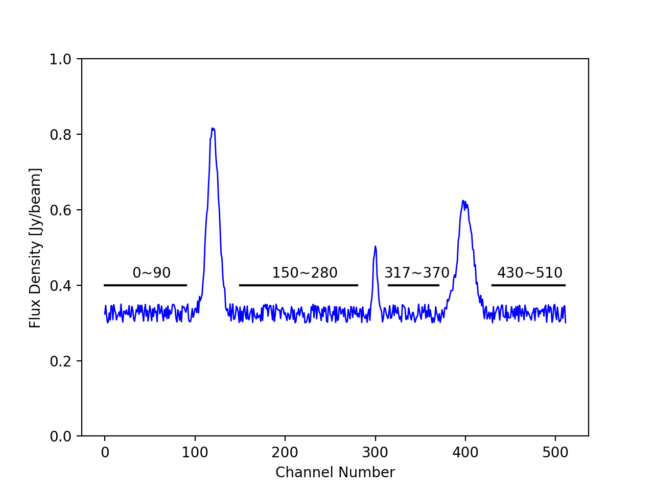
For this case the line free channel are 0 to 90, 150 to 280, 317 to 370 and 430 to 510. In CASA syntax this would be written as
(where '[SPW No.]' would be replaced by the SPW number and remember these are not the values to use with our data).
For the case of ALESS49 things fairly simple as we only have one spectral window which shows emission, but beware there are at least two sources within the field with emission at different velocity (ergo different channel ranges!). Inspect your newly created cubes as
Using the line free channel values you find we will use the CASA task uvcontsub to fit a continuum level and subtract it directly from the visibility data.
To do this enter the line free channel values in to the 'fitspw' parameter of uvcontsub at mystep = 0 in the script. For spectral windows with no line emission we need to include the whole SPW in this 'fitspw' parameter, separating each SPW with a comma in CASA syntanx.
The uvcontsub command looks like this:
field = 'ALESS49',
fitspw = [values you have found from inspecting the data],
want_cont=False)
You can then set mysteps=[1] and then execute the script.
This will create the measurement set 'ALESS49_ALL_EBS.ms.contsub'. We will use this in the imaging of spectral lines in the next step.
STEP 2: IMAGE A LINE
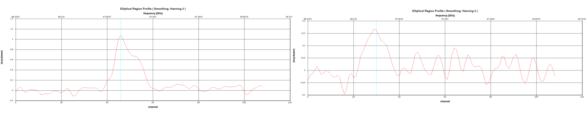
For this example we will use a line of CO found in spectral window 1 (see Figure X)
As we want to just image the line we will need to alter some parameters into our next tclean command. Those are:
nchan, the number of channels you wish to have in your cube, as we no longer want the whole frequency range.start, the start channel,frequency or velocity you wish to start you cube at. A few channels before emission is detected.width, the width of the individual channels within your cube. This must be in compatible units to the value you entered startstart. Here you can average up some channels by setting this > 1. However, I would recommend usingwidth=1for this example.
Based on the spectra in Figure 2 and 3 select your nchan, width and start values and enter them into the code at step = 2. When you have decided upon these values you can enter them into the relevant lines of code (again coloured red) in mystep = 2, which looks like this:
imagename = target+'_line_SPW1_contsubbed',#- Or whatever you would like to call the output image
field = target,
stokes = 'I',
spw = '1',
outframe = 'BARY',
restfreq = restnus[1],
specmode = 'cube',
imsize = [X, Y],#- You can use the previously calculated values here.
cell = 'Z.Aarcsec',#- You can use the previously calculated values here.
deconvolver = 'hogbom',
niter = 10000,
weighting = 'briggs',
robust = 0.5,
gridder = 'standard',
pbcor = True,
threshold = 'Q.VmJy',
width = '000.00kHz',
start = '000.00GHz',
nchan = W,
interactive = True)
You can then set mysteps=[2] and then execute the script. Again this will start an interactive clean, where you can draw a clean box around emission in each channel of the cube.
ASIDE: Auto-masking
You'll quickly see that drawing clean boxes can be very time consuming! But thankfully CASA recently introduced an Auto-masking option. Automasking (called by settingusemask='auto-multithresh') uses various user defined thresholds to 'mimic' what an experienced user would do when drawing clean boxes. The definitions of the threholds and the effects of changing them are described in detail in the Automasking CASA guide which can be found here: https://casaguides.nrao.edu/index.php/Automasking_Guide
STEP 3: IMAGE MOMENTS
Using the cube generated in Step 2 we can start to preform some image analysis. A useful task for this is immoments. This task allows you generate images of the -1th moment (mean value in spectrum), 0th moment (integrated intensity) up to the 11th moment (coordinate of the miminum pixel in the spectrum, apparently). (Note some of these moments have the typical mathematical meaning, where as some are more like convenience functions).
The most commonly used moments for image analysis are 0, 1 and 2 which are 'integrated value of the spectrum', 'intensity weighted coordinate' and 'intensity weighted dispersion of the coordinate'. The latter two are commonly used to infer 'velocity fields' and 'velocity dispersion' in the source. To generate such images for ALESS49 we call immoments as follows (see also step = 3 within the script):
moments=[0,1,2],
outfile='ALESS49_CO.I.manual.image.mom',#- Or whatever you would like to call the output image
excludepix=[X,Y],
chans='z~w')
For this task you need to set the channels over which you want to collapse the image to generate the moments using the chans parameter. It is also useful to set values in either includepix or excludepix, either of these parameters can be used (but not both) to limit the pixel values used in the generation of the moment images. includepix will allow immoments to use only pixel from a low value threshold (e.g. a few times the RMS noise) to a high value and conversely excludepix will only allow use of pixels from a very low value to a high value cut off (again e.g. a few times the RMS noise).
Once have set the red values above in the script you can mysteps=[3] and then execute the script.
STEP 4: EXPORT TO FITS FILE
Possibly the least exciting step, but as you will have seen CASA images are in the CASA image format, which is essentially a directory structure. This is fine if we want to work solely in CASA for all our analysis and will be sharing our results with other who will exclusively use CASA. However, it is more that likely that your colleage/supervisor/tame theorist will ask for an image as a FITS file, (the standard image format for most astronomical images) to use in another package. CASA has the task exportfits which allows us to do this.
In its simplest form you can export a FITS file with the following code:
fitsimage=yourImage+'.fits')
There are however a few things to keep in mind which might be useful when trying to get your CASA exported FITS file to be loaded properly in external packages. This is due to the fact that by default CASA images have 4 axis, which are listed in the following order:
- Axis 1 = x spatial axis,
- Axis 2 = y spatial axis,
- Axis 3 = Stokes axis (I Q U V),
- Axis 4 = frequency axis,
All four typically exist even if they have a value of 1 (i.e. Stokes 'I' only and 1 frequency plane).
Many other packages expecft either the Stokes and Frequency axes to be reversed or for the Stokes axis not to exist at all. To over come this issue exportfits has a few of parameters to deal with this. dropstokes = True will drop the Stokes axis entirely, dropdeg = True will drop any axes which have a length of 1 and stokeslast = True will put ensure that the Stokes axis is the last (rather than 3rd) axis in the exported FITS.
mystep=[4] in the code has an example of this.
Finally, if you have any problems then here is a version of the script with the all the answers in: scriptForSpectralLineImaging_withanswers.py