Simple Continuum Imaging

At the end of Simple continuum Calibration you made uid___A002_Xba4d35_Xb297.ms.split.cal, containing the calibrated data just for the targets. You can use your version, or if you did not get that far, download it as below; you will also need the script in any case.

wget -c http://almanas.jb.man.ac.uk/alma/Web/Meetings/2018/DurhamSchool/uid___A002_Xba4d35_Xb297.ms.split.cal.tar
wget -c http://almanas.jb.man.ac.uk/alma/Web/Meetings/2018/DurhamSchool/scriptForImagingBlanks.py

The script just contains one task which will be used (initially) to clean just one target, interactively. You will need to edit it so make a copy first just in case.

#for t in range(len(tgts)):      # This would loop through all targets listed in the script
for t in range(1):               # just the first field as a test starter
  os.system('rm -rf '+tgts[t]+'_sci.spw0_1_2_3.mfs.I.manual*')
  tclean(vis = thevis,
         imagename = tgts[t]+'_sci.spw0_1_2_3.mfs.I.manual',
         field = tgts[t],
         stokes = 'I',
         spw = '0,1,2,3',
         specmode = 'mfs',            # multi-frequency-synthesis produces one continuum image from all channels
         imsize = [isz, isz],
         cell = c,
         deconvolver = 'hogbom',      
         niter = 100,                 # increase for bright sources
         cycleniter=10,               # increase for bright sources
         weighting = 'briggs',       
         robust = r,
         mask = '',
         gridder = 'standard',
         pbcor = True,               # produce two images, one divided by the primary beam response.
         threshold = sig,
         interactive = True
         )

These are the parameters you are most likely to want to change. ? means fill in for yourself.

thevis = ['?']         # Calibrated MS to be imaged 
active=True            # whether to clean interactively or not
c = '?arcsec'          # pixel size  
isz = ?                # image size in pixels
r = 0.5                # robust parameter value  
sig = '250.e-6Jy'      # expected stopping threshold

Notes on parameter values

The pixel, or cell size is chosen to give at least 5 pixels across the synthesised beam. The synthesised beam is roughly given by (wavelength/longest baseline), the exact value depending on uv coverage and weighting. The listobs output from the calibration script gives the frequency and hence wavelength, λ, and the plots of uv coverage or uv distance give you the longest baseline, B (both in metres). CASA has built-in python maths, so you can just type

(3600.*degrees(λ/B))/5.

to get a value in arcsec to go in c.

Standard ALMA processing gives an image size up to 2x the primary beam FWHM, but since you know these sources are compact and have reasonably good positions (say, better than 5 arcsec) you can just image the central 8-10 arcsec to begin with. Work out how many pixels this needs and then set isz to the nearest well-factorizable number (this speeds the Fourier Transform part of cleaning; 360 or 512 are good examples). Also see how that compares to the FWHM, given in arcsec by 1.13*degrees(λ/D) where D is the diameter of each telescope, here 12 m.

The values of robust are in the range [-2, 2], where -2 is uniform weighting, for the highest resolution but the equal weight given to poorly-sampled regions usually gives worse beam sidelobes and increases the noise. The default for ALMA is 0.5, as, for good central uv coverage, this gives good resolution and minimises sidelobes. However if you want to increase the sensitivity to faint, extended emission you might try natural weighting (robust = 2) or even a uvtaper. If there is time, experiment with different values of robust and we can discuss tapering.

The stopping threshold is usually initially set to the predicted thermal map noise. From listobs, you can get the time on source per target and the other parameters needed by the ALMA Sensitivity Calculator. Really, the threshold should be the minimum flux needed to produce sidelobes, i.e. a few times the noise, and when cleaning interactively you might stop sooner, but it is worth remembering that if the weather was very dry and stable or you were at a frequency where the receivers perform very well, you might reach lower noise anyway. Conversely, without self-calibration, you would not expect a dynamic range better than a few hundred at most (or worse for sparse uv coverage).

Interactive cleaning

tclean Fourier transforms the chosen visibilities and displays a dirty image

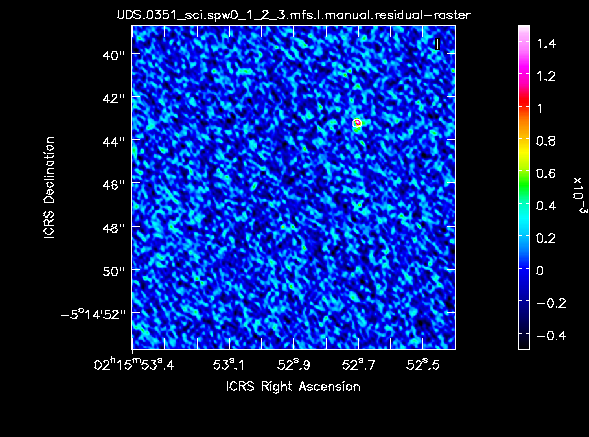
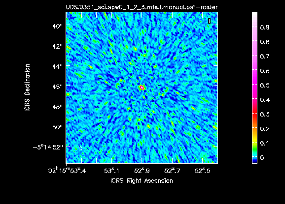
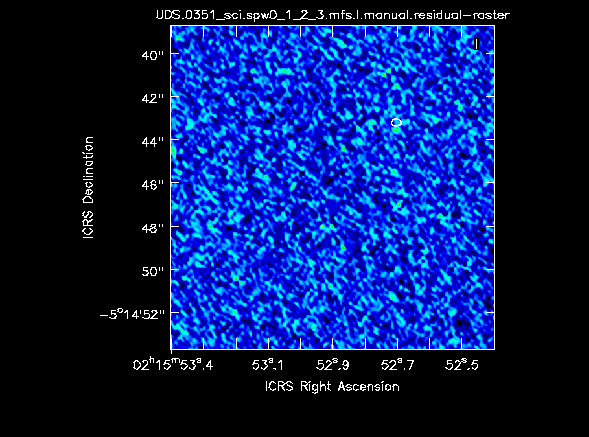
Use the ellipse (or rectangle or polygon) tool to draw a mask tightly enclosing any obvious source(s) and double-click inside the mask to activate it. tclean will select peaks within the mask, calculate the dirty beam response to a fraction of each, and subtract the emission. The peak parameters are stored as a table of Clean Components. This is performed for cycleniter iterations (a minor cycle) and the CC are then subtracted from the data in the uv plane and the residual image is displayed as shown below, alongside the dirty beam (Fourier transform of the uv tracks)/

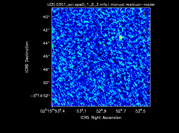
If necessary modify the mask and continue cleaning until the residuals look like pure noise.

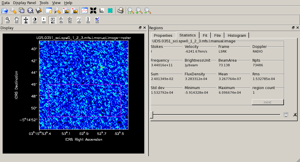
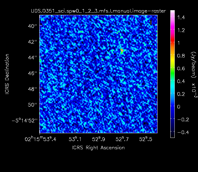
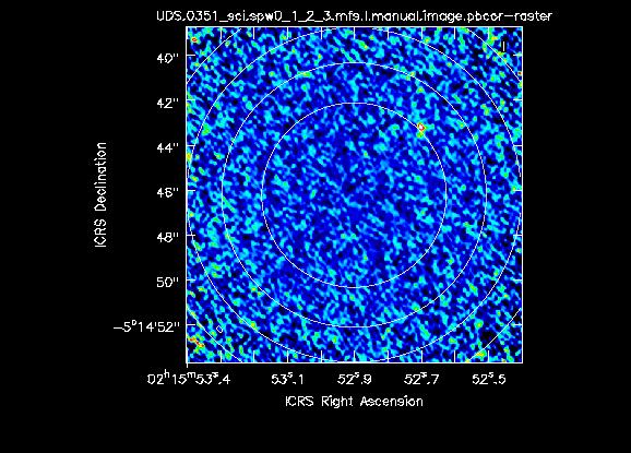
Press the red stop button, and when tclean has finished, use the viewer to display the cleaned .image. These plots also show the primary-beam corrected image, with contours at 0.8, 0.6, 0.4 of full sensitivity, and a zoom showing the CC superimposed.

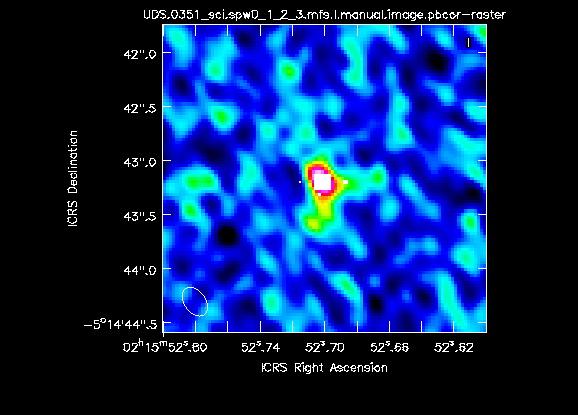
You can measure the rms (or the peak) of a chosen area in the viewer as shown (later we will show how to script this)