
ALMA Data Reduction: AS2UDS Basic
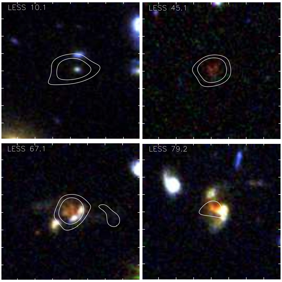
Previous ALMA results from ALESS
This page provides and explains the CASA commands needed to calibrate and image a set of observations. A companion page and scripts contain missing parameters to provide problem solving practice.
Preparation
These steps have been done for you already
CASA 4.5 is installed on each workstation and your ~/.casa/init.py has been set up to provide access to helper scripts called analysisUtils.
This guide uses ALMA data taken for project 2012.1.00090.S, which is now public domain and can be downloaded from the ALMA Science Archive via the Portal. These data were obtained with the 'Include raw' switch, in order to allow tweaking the calibration. This gives:
| 2012.1.00090.S_uid___A002_X5eed86_X27_001_of_001.tar | 375M |
| 2012.1.00090.S_uid___A002_X5eed86_X2b_001_of_001.tar | 378M |
| 2012.1.00090.S_uid___A002_X7143f6_Xca4.asdm.sdm.tar | 4.0G |
| 2012.1.00090.S_uid___A002_X7143f6_Xf9b.asdm.sdm.tar | 4.0G |
Data reduction requires a directory with at least 60 G free space (to avoid having to delete intermediate steps). Each file has been un-tar'd using
tar -xvf 2012.1.00090.S_uid___A002_X5eed86_X27_001_of_001.tar
etc., which puts all the files into the correct directory structure. The files called *asdm.sdm are the raw data in Science Data Model format, which is very compact for transport but not accessible for calibration. They have been renamed to drop the suffix to comply with the input format for the task which converts them to Measurement Sets (a bulkier but more accessible format). The ASDM/MS are usually referred to by their last unique identifier, here Xca4 and Xf9b.
Each of the two data sets (Xca4 and Xf9b), contains a short observation of a bandpass calibrator and a flux scale calibrator, and then a series of interleaved scans on one phase reference source and a series of targets within 15 degrees. We will go through Xca4 together first and then you can have a look at Xf9b where the script has been modified to provide problem-solving practice.
Getting started
The parent data directory is 2012.1.00090.S. You can explore this or go straight to:
cd Durham/AS2UDS/2012.1.00090.S/science_goal.uid___A002_X5eed86_X25/group.uid___A002_X5eed86_X26/member.uid___A002_X5eed86_X27/
emacs README &
This describes what is in the data delivery and how to re-create the calibrated data.
cd script
ls
emacs uid___A002_X7143f6_Xca4.ms.scriptForCalibration.py &
Usually, you can assume that the calibration is good and just run this as per the instructions using scriptForPI.py, but we want to examine each process so we will go through the basic script uid___A002_X7143f6_Xca4.ms.scriptForCalibration.py step by step. This has been modified in a few places to make it compatible with the current version of CASA.
cd ../raw
ls
You will see uid___A002_X7143f6_Xca4
Instrumental calibration
Check that you are in directory Durham/AS2UDS/2012.1.00090.S/science_goal.uid___A002_X5eed86_X25/raw. Start CASA:
 /local/scratch/amsr/chantico_2/Durham/casa-release-4.5.0-el6/casapy
*******************
Convert data to MS format, list contents of MS
You see that uid___A002_X7143f6_Xca4.ms.scriptForCalibration.py is structured so that you can choose which processes to run as in the example below. It also contains a list of source names, roles and numbers.
# In CASA:
mysteps=[0, 1, 2]
execfile('../script/uid___A002_X7143f6_Xca4.ms.scriptForCalibration.py')
Step 0 converts the ASDM to Measurement Set format, Step 1 corrects minor labelling bug, and Step 2 lists the contents of the MS.
# In CASA:
!ls                 # Use any shell command prefixed by !
!emacs uid___A002_X7143f6_Xca4.ms.listobs &
which shows
uid___A002_X7143f6_Xca4.ms
uid___A002_X7143f6_Xca4.ms.flagversions
uid___A002_X7143f6_Xca4.ms.listobs
We will go through the contents listing.
Apply initial flags
# In CASA:
mysteps=[3]
execfile('../script/uid___A002_X7143f6_Xca4.ms.scriptForCalibration.py')
This applies flags generated by the on-line system e.g. pointing scans, since the pointing offsets are applied in real time, and dead time between scans (see plot which will appear). Don't worry about a few error messages, these are connected with the problem fixed in Step 1.
Water Vapour Radiometry corrections
# In CASA:
mysteps=[4]
execfile('../script/uid___A002_X7143f6_Xca4.ms.scriptForCalibration.py')
This step reads the measurements taken using the 183-GHz Water Vapour Radiometers (WVR) and uses them to calculate the residual delay fluctuations due to variations in precipitable water vapour (PWV) above each antenna, and thus phase corrections. The parameters allow the same corrections to be applied to the phase reference and target sources, along with heuristics to compensate for any anomalous measurements. The corrections are written to the uid___A002_X7143f6_Xca4.ms.wvr calibration table, as well as a diagnostic file and plots.
This task, wvrgcal was originally run with default inputs. Look at the preliminary diagnostic plots of WVR phase corrections, which show that the data for DV09 are very noisy. The inputs to wvrgcal were modified to flag those WVR data and interpolate from the nearest 3 antennas. You can see this in the script or you can inspect the inputs to any CASA task using the following:
# In CASA:
default(wvrgcal)         # re-initialises the task
inp wvrgcal              # shows default inputs

tget(wvrgcal)            # restore settings from last successful execution
inp wvrgcal
We will talk through the inputs.
Inspect the plots and the diagnostic table.
# In CASA:
!gthumb uid___A002_X7143f6_Xca4.ms.wvr.smooth.plots/*png &
!emacs uid___A002_X7143f6_Xca4.ms.wvrgcal &
Inspect uid___A002_X7143f6_Xca4.ms.wvrgcal to find the PWV during observations. Look at uid___A002_X7143f6_Xca4.ms.wvr.smooth.005.png (or see Phase corrections derived from WVR for a range of baseline lengths). Why are there stronger variations on some baselines?
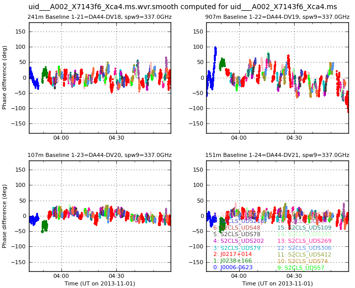
Phase corrections derived from WVR for a range of baseline lengths
Tsys corrections
# In CASA:
mysteps=[5]
execfile('../script/uid___A002_X7143f6_Xca4.ms.scriptForCalibration.py')
This step checks the (per-channel) Tsys measurements and uses them to write the uid___A002_X7143f6_Xca4.ms.tsys calibration table. Inspect the plots:
# In CASA:
!gthumb  uid___A002_X7143f6_Xca4.ms.tsys.plots.overlayTime/
There are no ridiculously high values or bad spikes, so these corrections are good. If there were bad values, you should check the data themselves (see plotms below) and if it is only the Tsys which is bad, follow the link at the bottom of analysisUtils to Todd's wikipage, which contains utilities to fix this.
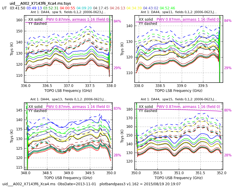 Tsys corrections for one antenna
 Antenna position corrections
# In CASA:
mysteps=[6]
execfile('../script/uid___A002_X7143f6_Xca4.ms.scriptForCalibration.py')
When this data reduction script was generated, the parent script searched the antenna moves database to see whether any position corrections had been updated since the observation date (but while the antennas used were still on the same pads). As none were found, the correcttion table is blank but is included to allow the next applycal step to be standard.
Apply instrumental corrections, split out, list and inspect the corrected data
# In CASA:
mysteps=[7, 8, 9]
execfile('../script/uid___A002_X7143f6_Xca4.ms.scriptForCalibration.py')
After checking the WVR and Tsys tables, these corrections are applied, interpolating in time/between phase-ref and target as required. If you look at the .listobs file again, you will see that the science spectral windows (un-averaged channels, at Band 7 frequencies) are 9, 11, 13, 15 and these are the ones which are calibrated and then split out. If you were really short of space, you could estimate whether you could do any channel- or time-averaging without smearing within your field of view, and perform some averaging in split, but we don't need to here.
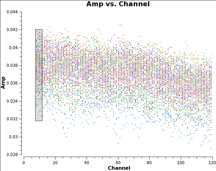
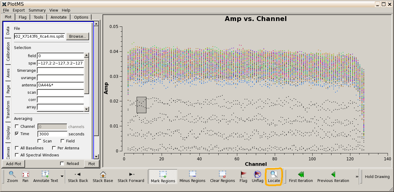 Raw bandpass calibrator data after excluding first two channels, and the identification of bad data
List your directory contents to see the new file uid___A002_X7143f6_Xca4.ms.split and open uid___A002_X7143f6_Xca4.ms.split.listobs in a text editor. Now there are just 4 spw, numbered 0-3, containing the science data. The 'DATA' column of the MS has the data with the Tsys and WVR corrections applied.
The refant is chosen to be the origin of phase; that is, the corrections are calculated assuming that its phase is consistently zero. It should be an unshadowed antenna with good data near the centre of the array so that its baseline lengths are minimised, making it easier to find solutions. The script generator selected DA44, is that a good choice?
# In CASA:
default(plotants)
vis      = 'uid___A002_X7143f6_Xca4.ms.split'
inp
plotants()                # Typing the name of the task will run it
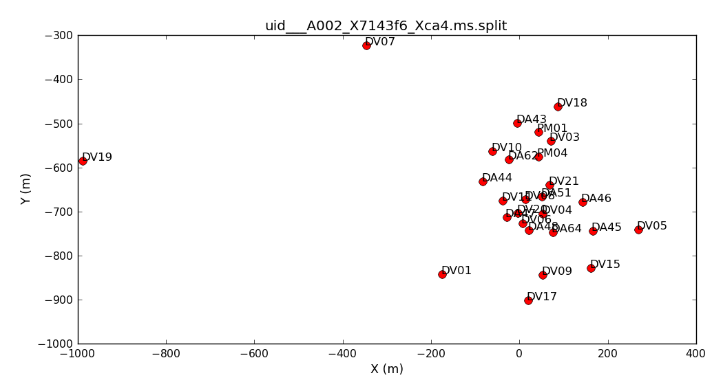 Antenna positions
Inspect the data:
# In CASA:
plotms(vis='uid___A002_X7143f6_Xca4.ms.split',
	field='0',     # the bandpass calibrator, see listobs output
	xaxis='channel', yaxis='amp',
	antenna='DA44&*', # plot all baselines to refant
	coloraxis='baseline',
	avgtime = '3000s')
You see that the first few channels are very wild. In the spw box enter
0:2~127,1:2~127,2:2~127,3:2~127
to exclude these, and hit plot You now see, firstly, that there are more low-sensitivity channels at the high end of each spectral window and that there are also some bad data. Use mark and locate and you will see that these are all DV06. If you now inspect the inputs for Step 10 you see that the end channels will be flagged, as well as DV06. Periods where one antenna is shadowed (i.e. is pointing at the back of another nearby) are also automatically detected and flagged.
Calibration using astrophysical calibration sources
From here on, 'raw' means with WVR and Tsys corrections applied, but no further calibration.
Apply flags and set flux standard
# In CASA:
mysteps=[10, 11, 12]
execfile('../script/uid___A002_X7143f6_Xca4.ms.scriptForCalibration.py')
These data use a QSO as the flux scale standard. A few dozen sources are monitored regularly (every few weeks) by ALMA so the measured flux density is within a few percent of the true value. However, when this script was originally generated, we did not think that we were accurate enough to bother about the spectral index. We now know that it is worth it, so adjust the values as follows:
Listobs gives you the date of observation, which is needed in the format YYYY-MM-DD. Listobs, or in this case the inputs for setjy, give you the central frequencies of each spectral window (spw). Use a utility as follows:
# In CASA:
# use frequency for spw 0
aU.getALMAFlux('J0238+166','336.994575GHz',date='2013-11-01')
This returns
'fluxDensity': 0.610058
'spectralIndex': -0.4518
These values have been used to update the script, and the 'manual' option (a new parameter in setjy) has been inserted. Inspect the model:
# In CASA:
plotms(vis='uid___A002_X7143f6_Xca4.ms.split',
	field='1',     # the flux standard
	xaxis='frequency', yaxis='amp',
        ydatacolumn='model')
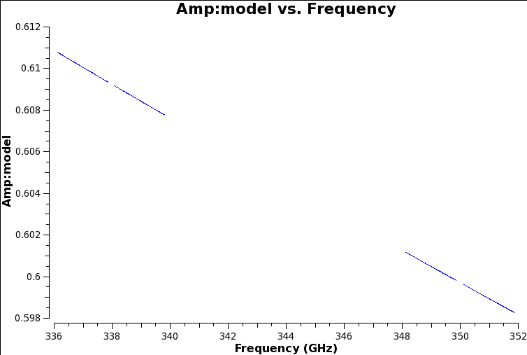 The model set for the flux standard
Steps 10 and 12 apply the flags and back up the existing flagging state. Applying the calibration later can cause more data to be flagged; this step allows you to return to the pre-calibration state. Check your flag version names:
# In CASA:
!ls uid___A002_X7143f6_Xca4.ms.split.flagversions/
Bandpass calibration
# In CASA:
mysteps=[13]
execfile('../script/uid___A002_X7143f6_Xca4.ms.scriptForCalibration.py')
The atmosphere is the main factor which causes the signal amplitude and phase to vary on short timescales, whilst there are similar variations across the band as a function of frequency primarily due to instrumental effects.
Plot the (edited) bandpass, just one polarization for clarity:
# In CASA:
plotms(vis='uid___A002_X7143f6_Xca4.ms.split',
	field='0',     # the bandpass calibrator, see listobs output
	xaxis='channel', yaxis='amp',
	correlation='YY',
	antenna='DA44&*', # plot all baselines to refant
	coloraxis='baseline',
	avgtime = '3000s')
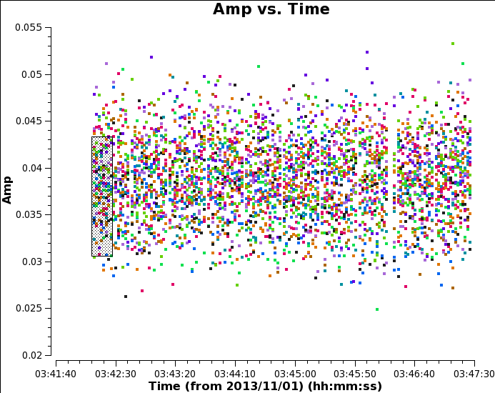
Use the select tool to mark the extent of a short time segment (as in the figure Raw, time-averaged data for bandpass calibrator), then deslect time averaging and plot again. You will see that although with no averaging the scatter is greater, the mean flux density is higher. This is because when we averaged all times, we were averaging a changing phase. You can see this if you plot phase against time:
# In CASA:
plotms(vis='uid___A002_X7143f6_Xca4.ms.split',
	field='0',     # the bandpass calibrator, see listobs output
	xaxis='time', yaxis='phase',
	spw='0',
	correlation='YY',
	antenna='DA44&*', # plot all baselines to refant
	coloraxis='baseline',
	avgchannel = '128')
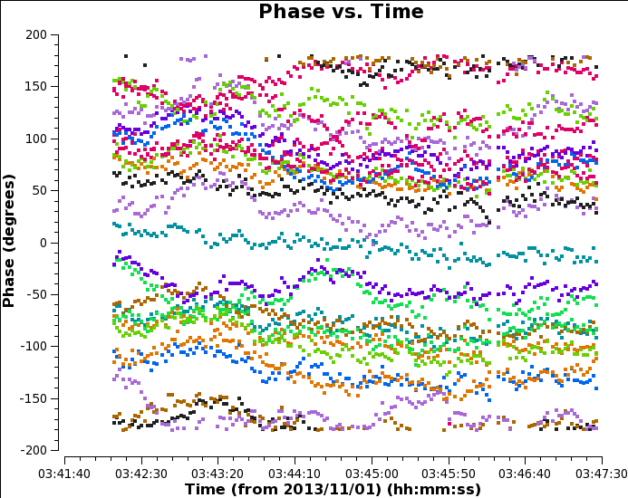
Averaging the phase change across all channels produces a lower amplitude v. time than just averaging a few channels
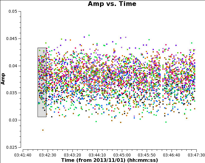
Thus, in order to minimise decorrelation, first just a few channels in the centre of each spw are averaged to calibrate the bandpass calibrator phase and amplitude as a function of time. The corrections are then applied 'on the fly' in order to derive the bandpass corrections. This allows averaging of all times on the bandpass calibrator source to get enough signal to noise to solve per-channel.
In each case, the algorithms used by gaincal and bandpass use a model in the measurement set to compare with the actual data, and work out (using a least squares or other chi-squared minimisation method) the corrections to be applied per antenna, in order to make the actual data as much like the model as possible. Here, we are assuming that the calibration sources are point-like, so the model has zero phase. For the sources of unknown flux density the default model is a 1 Jy source at the phase centre.
Look at the inputs to gaincal in CASA (or in the script):
# In CASA:
tget(gaincal)
inp
The parameters which have to be set here include:
vis      = 'uid___A002_X7143f6_Xca4.ms.split'                 #  Name of input MS
caltable = 'uid___A002_X7143f6_Xca4.ms.split.ap_pre_bandpass' #  Name of output gain table

field    = '0'                     # Name or number of bandpass calibration source
spw      = '0:51~76,1:51~76,2:51~76,3:51~76' # Central channels to avoid decorrelation
refant   = 'DA44'
Inspect the plots of the time-dependent pre-calibration and the bandpass calibration itself:
# In CASA:
!gthumb uid___A002_X7143f6_Xca4.ms.split.ap_pre_bandpass.plots/* &
!gthumb uid___A002_X7143f6_Xca4.ms.split.bandpass.plots/* &
These should show fairly smooth solutions (as indeed they do). DA44 has flat, zero phase solutions because it is the reference antenna.
Time-dependent calibration of phase and amplitude
# In CASA
mysteps=[14, 15]
execfile('../script/uid___A002_X7143f6_Xca4.ms.scriptForCalibration.py')
Phase solutions v. time (per integration)
After another flag back-up, gaincal is used to derive phase solutions, per integration, as a function of time. The bandpass table is applied so all channels can be averaged. The spw and polarizations are kept separate since atmospheric delays and instrumental effects may corrupt these differently (although in the case of spw, the bandpass calibration should have taken care of that). If you scroll back (or search) in the logger, you will see
Calibration solve statistics per spw (expected/attempted/succeeded):
Spw 0:996/630/630
There are fewer 'attempted' than 'expected' because some data have been flagged, but all of those 'attempted', 'succeeded'. If more than ~10% failed you could look and see whether it was bad data (needing flagging) or just low signal to noise. If the latter, you could (just for the source in question) average for longer in time, say 30s, or average spw.
# In CASA
!gthumb uid___A002_X7143f6_Xca4.ms.split.phase_int.plots &
There are likely to be jumps between sources but the phase reference solutions should track smoothly.
Amplitude solutions v. time (per scan)
Now, these phase solutions (and the bandpass table) are applied in order to derive amplitude solutions per scan (that is what solint 'inf' means unless you explicitly select scan averaging). The amplitude errors are usually slower-varying and one needs better signal to noise for good solutions, hence the longer averaging time than for phase.
# In CASA
!gthumb uid___A002_X7143f6_Xca4.ms.split.ampli_inf.plots &
Deriving calibrator source flux densities
We have set the flux densities of our flux standard, but the other two calibration sources (the bandpass and phase reference calibrators) have the default models of 1. The next step is the task fluxscale, which uses the corrections for the flux standard to estimate the factors needed to multiply the gains for the other two sources to calculate their flux densities on the same scale and writes a scaled table uid___A002_X7143f6_Xca4.ms.split.flux_inf. You can inspect the values in a log file:
# In CASA
!emacs uid___A002_X7143f6_Xca4.ms.split.fluxscale &
These should have good SNR and be consistent from spw to spw with a sensible spectral index.
Phase solutions v. time (per integration)
Finally, we derive another phase-only solution table with solint 'inf'. The first set of solutions, solint 'int' were best for correcting the calibrators themselves, but averaging the solutions for each phase reference scan minimises the phase noise included in interpolating these onto the target.
# In CASA
!gthumb uid___A002_X7143f6_Xca4.ms.split.ampli_inf.plots &
Apply calibration and split out the corrected data
# In CASA
mysteps=[16, 17]
execfile('../script/uid___A002_X7143f6_Xca4.ms.scriptForCalibration.py')
After saving flags again, these tasks apply the calibration and split out the calibrated data. Have a look at the inputs to applycal in the script and, for the last use, as below:
# In CASA
tget(applycal)
inp
vis    = 'uid___A002_X7143f6_Xca4.ms.split'
field  = '2,3~17' # 2 is the phase-reference and the others are the targets.
gaintable  = ['uid___A002_X7143f6_Xca4.ms.split.bandpass', 'uid___A002_X7143f6_Xca4.ms.split.phase_inf', 'uid___A002_X7143f6_Xca4.ms.split.flux_inf']
gainfield      = ['', '2', '2']
The gainfield parameter specifies which source in each gain table will provide the solutions to be applied (to all the fields specified). The bandpass calibration table (the first in the list) was derived from just one source so there is no need to specify the gainfield, but we want to make sure that the time-dependent solutions for the phase-reference are selected and applied to itself and to the target (since uid___A002_X7143f6_Xca4.ms.split.phase_inf and uid___A002_X7143f6_Xca4.ms.split.flux_inf contain solutions for all calibration sources).
Inspect the calibrated data:
# In CASA
plotms(vis='uid___A002_X7143f6_Xca4.ms.split',
	field='0',     # the bandpass calibrator, see listobs output
	xaxis='time', yaxis='phase',
	ydatacolumn='corrected',
	coloraxis='spw',
	avgchannel = '128')
Repeat for the phase-ref, field 2 and plot its amplitudes also.
They all look level and close to the expected value.
Check that the phase-ref is point-like:
# In CASA
plotms(vis='uid___A002_X7143f6_Xca4.ms.split',
	field='2',     # phase ref
	xaxis='uvwave', yaxis='amp',
	ydatacolumn='corrected',
	coloraxis='spw',
	avgchannel = '128')
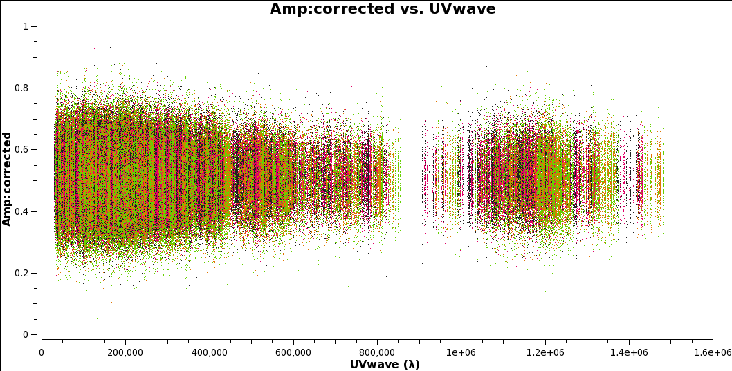
Note the maximum uv distance and the distance before the big gap. You will need these values later.
Imaging the targets
Interactive cleaning
The scriptForImaging.py is similar to a standard imaging script, with some modifications, made with the benefit of hindsight, for speed. First, though, we will image a target interactively in order to see what is involved.
# In CASA
default(clean)
inp clean
Most of the paramters we need are fairly obvious but here are some explanations:
cell is the pixel size. This should give at least 3, usually ~5, pixels across the synthesied beam (resolution), and we calculate that from the maximum uv distance noted above. This is simply the longest baseline, in units of observing wavelength, i.e. (B in metres)/(lambda in metres). (For information, the observing wavelength is around 0.9 mm and the longest baseline was just under 1.4 km.)
The resolution in radians is then given by (lambda/B) or (1/max. uv distance in lambda). Say this was 1.5E+6 lambda (wavelengths), then, converting to arcsec, you can type:
# In CASA
3600.*degrees(1./ 1.5E+6)
giving 0.14 arcsec. 0.03 arcsec is a reasonable cell size.
Initially, we set the total image size to be about the FWHM of the antenna primary beam, given by:
# In CASA
cell = 0.03              # pixel size in arcsec
wavel=0.0009             # wavelength in m (NB lambda is a 'reserved' variable, don't use)
PB   = 12.               # antenna diamter in m
FWHM=3600.*degrees(1.12*(wavel/PB))
FWHM
imagesize = FWHM/cell
imagesize
In fact, we will set imagesize to 512 as certain numbers are preferred for efficiency in the Fourier Transform steps.
# In CASA
os.system('rm -rf uid___A002_X7143f6_Xca4.ms.clean.source3*') # get rid of old images
default(clean)
inp

vis = 'uid___A002_X7143f6_Xca4.ms.split.cal'
imagename = 'uid___A002_X7143f6_Xca4.ms.clean.source3'
field = '3'               # S2CLS_UDS79
mode = 'mfs'              # Combine all frequencies for a continuum image
interactive = T           # Mask manually
imsize = [512, 512]
cell = '0.03arcsec'
weighting = 'briggs'
robust = 0.5

inp
Check that you understand each of the parameters you have set above (use help clean). weighting and robust control how the algorithm interpolates into the missing spacings in the visibility plane. robust +2/-2 correspond to completely natural/uniform weighting respectively; 0.5 means that there is some interpolation with a lower weight into unsampled parts of the uv plane; this gives slightly higher resolution but supresses sidelobes for most ALMA configurations.
When you are ready:
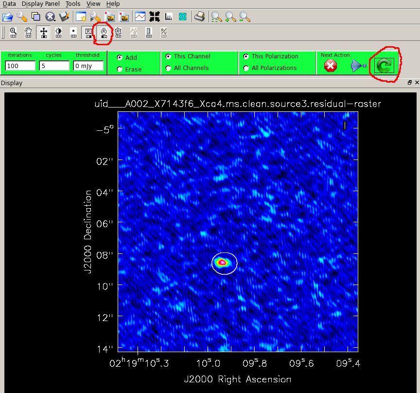
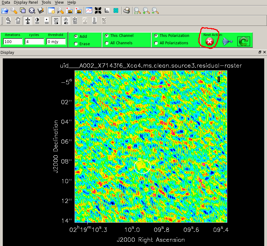
# In CASA
clean
and when the viewer appears, click on the ellipse to draw a mask around the emission. Double-click in the mask to activate it and click on the green arrow to start cleaning. After 100 interations the residuals are displayed again and as there is nothing brighter than the noise you can hit the red button to stop cleaning. Have a look at the messages in the logger. This tells you that the minimum and maximum residuals were similar in magnitude, and the beam size was about 0".32 by 0".22 (this is slightly larger than expected becuase, as plotants showed, there are very few very long baselines).
# In CASA
!ls -d uid___A002_X7143f6_Xca4.ms.clean.source3*    # list files clean created

viewer('uid___A002_X7143f6_Xca4.ms.clean.source3.image') # view image
Imaging all the fields and measuring basic properties
Take a look at ../script/scriptForImaging.py. This does what you have been doing, but instead of setting the mask interactively, it uses the masks made previously in QA2. This will not work if you change the directory structure, unless you alter the script as well. When ready:
# In CASA
execfile('../script/scriptForImaging.py')
When finished, inspect all the images the lazy way (NB don't try this for more than ~20 images at once).
# In CASA
ims=!ls -d *image   # pass the shell listing to a python variable

for i in ims:
  viewer(i)
You will see that several fields contain more than one source, which suggests that imaging a larger field of view might be useful. You also see that source 14 does not seem to have been detected, this will be investigated later.
The task imstat is used to measure the rms noise and the peak of each image. Since we don't know te exact position of each source, take the minimum of two boxes to measure the noise. You can have a look at the inputs and run the task interactively. Alternatively, the code below will pass the relevant part of the output of imstat to a python variable and format the numbers. This form of for loop could also have been used in the viewer, above.
You could copy the output to a text file - or if you kow some python, write it directly to a file.
# In CASA
for i in range(3, 18):
  rms1=imstat(imagename='uid___A002_X7143f6_Xca4.ms.clean.source'+str(i)+'.image', box='12,12,500,100')['rms'][0]
  rms2=imstat(imagename='uid___A002_X7143f6_Xca4.ms.clean.source'+str(i)+'.image', box='12,400,500,500')['rms'][0]
  print 'rms in uid___A002_X7143f6_Xca4.ms.clean.source'+str(i)+'.image: %6.3f mJy' %(1000.*min(rms1, rms2))
  peak=imstat(imagename='uid___A002_X7143f6_Xca4.ms.clean.source'+str(i)+'.image', box='12,12,500,500')['max'][0]
  pos = imstat(imagename='uid___A002_X7143f6_Xca4.ms.clean.source'+str(i)+'.image', box='12,12,500,100')['maxposf'][0:27]
  print 'Peak in uid___A002_X7143f6_Xca4.ms.clean.source'+str(i)+'.image:  %6.3f mJy/beam \n(before primary beam correction), at %28s' %((1000.*peak) , pos)
  print 'Dynamic range in uid___A002_X7143f6_Xca4.ms.clean.source'+str(i)+'.image: %5.1f \n' %(peak/(min(rms1, rms2)))
More imaging
To detect source 14, we can try tapering the beam (reducing the weight of the longest baselines), which will improve the sensitivity to extended emission by increasing the synthesised beam; there is a compromise between this and downweighting so much data that the noise increases. The outertaper is set to the value which contains all but the sparsely-filled outermost spacings, noted from plotting the uv distance previously, but you can experiment with other tapers. We also increase the image size just in case.
# In CASA
os.system('rm -rf uid___A002_X7143f6_Xca4.ms.clean_taper.source14*')
clean(vis = 'uid___A002_X7143f6_Xca4.ms.split.cal',
  imagename = 'uid___A002_X7143f6_Xca4.ms.clean_taper.source14',
  field = '14', # S2CLS_UDS345
  spw = '0,1,2,3',
  mode = 'mfs',
  interactive = T,
  imsize = [1024, 1024],
  cell = '0.03arcsec',
  phasecenter = 14,
  weighting = 'natural',
  uvtaper=T,
  outertaper='800klambda')
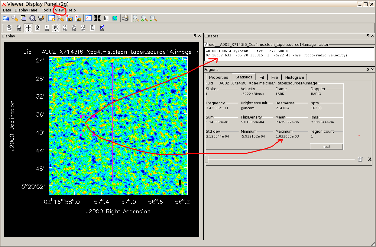
Note that the logger tells you the beam size is now 0".46 x 0".37. Use the viewer to inspect the image. You can measure the peak and noise interactively using the View - Cursor menu and the View - Regions menu, Statistics pane, see demo. Compare the noise, peak etc. with the previous image of this field. (The plot shows the measurements from hovering over the brightest point; hovering over the other box gives the off-source rms.)
Primary beam correction
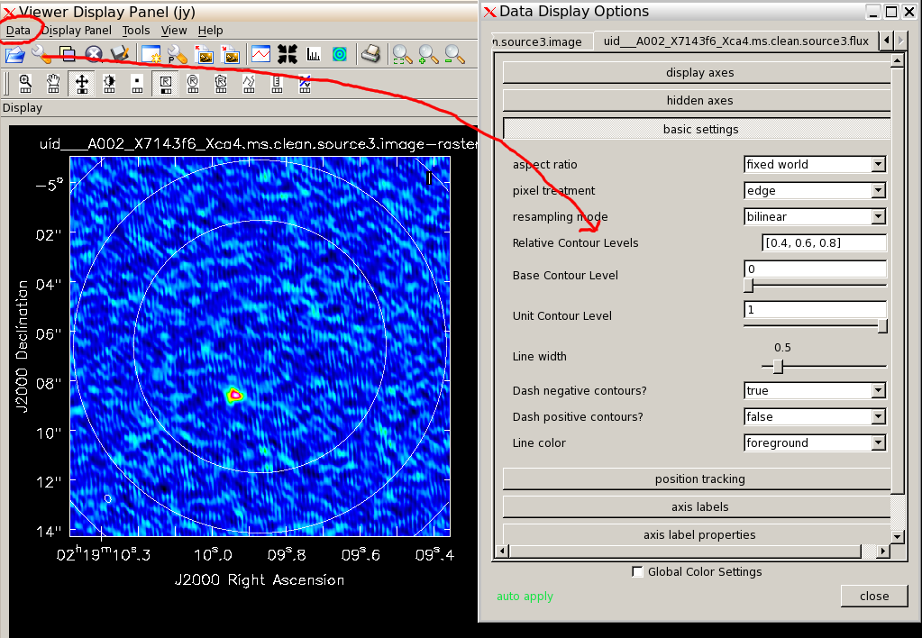
Display any one of the images and then use the Data - Open menu to overlay the primary beam contours from the .flux image (see demo and figure). Use the spanner icon to give you a menu which shows you the default contour vevels (you can change these).
# In CASA
viewer('uid___A002_X7143f6_Xca4.ms.clean.source3.image')
Apply the primary beam correction to all images. The loop below covers all the standard images; do the larger image of source 14 yourself.
# In CASA
for i in range(3, 18):
  impbcor(imagename='uid___A002_X7143f6_Xca4.ms.clean.source'+str(i)+'.image',
	pbimage='uid___A002_X7143f6_Xca4.ms.clean.source'+str(i)+'.flux',
	outfile='uid___A002_X7143f6_Xca4.ms.clean.source'+str(i)+'.pbcorr')
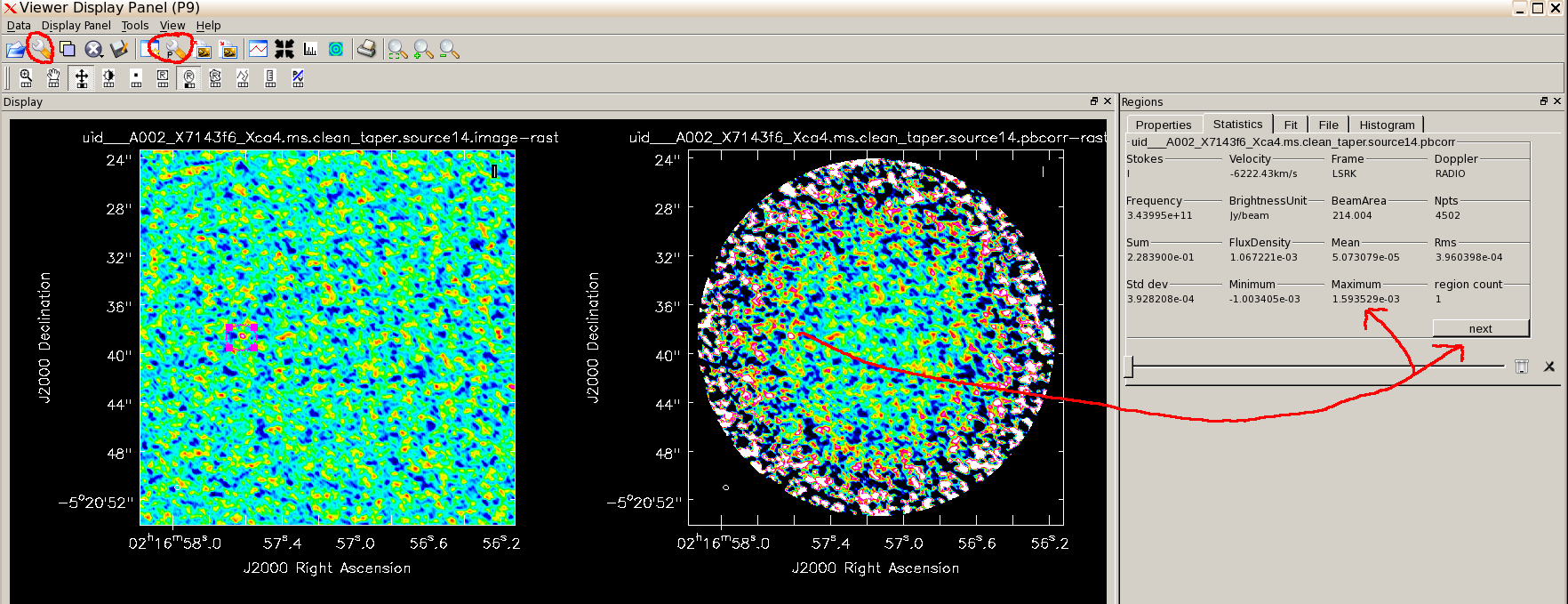
Display the uncorrected, tapered image for source 14. Open the Data Display Options menu using the spanner icon and select Global Color Settings (at the bottom). Using the other (!) P-spanner icon to open the primary-beam corrected image. You can again use View - Regions - Statistics to measure the peak etc.; draw the box on the first image and use the 'next' button to toggle between measurements for the two images. You see that the actual flux density of our putative peak has increased by about 50% thanks to the primary beam correction.
It is best to measure the SNR before applying the primary beam correction, because otherwise you have to measure the rms at the same radius as the source, but you can see that some of the sources are far enough out for this to make a difference to the actual flux density.
# In CASA
for i in range(3, 18):
  viewer('uid___A002_X7143f6_Xca4.ms.clean.source'+str(i)+'.pbcorr')
  peak=imstat(imagename='uid___A002_X7143f6_Xca4.ms.clean.source'+str(i)+'.pbcorr', box='12,12,500,500')['max'][0]
  print 'Peak in uid___A002_X7143f6_Xca4.ms.clean.source'+str(i)+'.image:  %6.3f mJy/beam \n(with primary beam correction)' %((1000.*peak))
Finally, write the images out as fits if you want to analyse them in other packages.
# In CASA
for i in range(3, 18):
  exportfits(imagename='uid___A002_X7143f6_Xca4.ms.clean.source'+str(i)+'.pbcorr',
  fitsimage='uid___A002_X7143f6_Xca4.ms.clean.source'+str(i)+'.pbcorr.fits')
This exports the standard but primary beam corrected images; you can write your own commands to export other images such as the larger Source 14. In more recent ALMA data releases, the primary beam correction and fits export are usually included in the imaging script.