Self-Calibration
This starts from the pipeline-calibrated data for 2017.1.00629.S RXCJ0439+05 observed on 2018-01-11. These data are still proprietary so please use only for teaching/testing. We provide input files which you can get as below in advance or from a USB drive on the day
wget -c http://almanas.jb.man.ac.uk/alma/Web/Meetings/2018/DurhamSchool/member.uid___A001_X1284_X3b5.hifa_calimage.weblog.tgz
wget -c http://almanas.jb.man.ac.uk/alma/Web/Meetings/2018/DurhamSchool/RXCJ0439_line.split.tar
wget -c http://almanas.jb.man.ac.uk/alma/Web/Meetings/2018/DurhamSchool/RXCJ0439.split.tar
wget -c http://almanas.jb.man.ac.uk/alma/Web/Meetings/2018/DurhamSchool/RXCJ0439_selfcalBlanks.py
The web log was already introduced, but if you missed it, gunzip it and in the file structure you will find index.html which you can open in a browser.
The target data consists of 4 spw, of which the 4th was originally in high spectral resolution. In RXCJ0439.split this has been averaged to the same resolution as the 3 continuum spw; RXCJ0439_line.split contains the central quarter of the line spw with less spectral averaging.
The script is set up to:
- 0 List the contents of the MSs and plot the data in plotms. The plots are designed to help you to estimate the S/N of the data on the longest baselines, to select the line-free channels and to consider a suitable interval for phase solutions. Make more plots interactively as you need.
- 1 Back up the initial flagging state (and add flagdata commands if wanted)
- 2 Make the first continuum image, with only phase-reference solutions applied, measure its S/N and insert the Fourier Transform of the Clean Components into the MS.
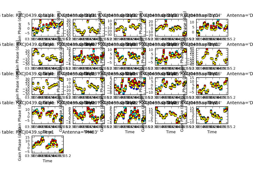
- 3 Use this as the model to compare with the continuum data and derive solutions in the first round of phase-only gaincal, and plot the solutions. Since this is a complex source, the solutions may vary more than for a phase-ref but they should not be random scatter.
- 4 Back up the flags again, apply the 'p' gain table and make another image etc. as in 2.
- 5 As 3 for amplitude self-calibration (applying the phase solution table)
- 6 As 4, applying both 'p' and 'a' solution tables
- 7 Apply the calibration to the line data and plotms to find the continuum-only channels
- 8 Use mstransform to fit and subtract the continuum from the line data
- 9 Select channels covering the line and image the cube,
You need to enter values for variables representing a number of parameters in the script; mostly you need to do this one step at a time as information from the previous step may be needed. Some tips:
Is the target bright enough to self-calibrate? The lazy answer is, yes the continuum looks really bright. Or to be more precise: if the flux density on the longest baselnes to the refant is P~100 mJy and the predicted map σrms(ttot) is 0.02 mJy, then for N=43 antennas, total time on target ttot ~ 21 min, you can estimate the minimum solution interval for 3σrms on each of 4 spw in 2 polarizations as:
dtmin ≥ 8x [3 x σrms(ttot)/P]2 tot.t x [(N(N-1)/(2(N-3))] < 1 sec so indeed plenty of signal (the data have been averaged to ~13 s integrations).
S/N = P/σrms(ttot) ~5000, which is a very high dynamic range and other errors e.g. residual bandpass errors. faint lines, may make it hard to reach this. It also means that you should fit for the source spectral index in cleaning after the initial phase corrections; even if the spectral index fitted is not very accurate it will improve the total intensity image quality.
Cleaning: For the first image, do not clean too deeply as you don't want to include spurious structure in the first model. Subsequently, make sure that you have all the flux in the model before you do amplitude self-cal. if you want you can experiment with automasking, see https://casaguides.nrao.edu/index.php/Automasking_Guide
Solution intervals: This is hard to estimate for a complex source where phase v. time may wiggle due to errors or to source structure, both affecting longer baselines more. The interval should be less than a change of ~π/4, but for the first round of self-calibration do not use a very short interval if the model may be not very accurate, as you don't want to impose detailed but incorrect structure (this can usually be calibrated out later if necessary but will requires more rounds of calibration). Anything from 30s up to a scan is typical for ALMA. Amplitude errors are more slowly-varying so a longer interval, typically a scan or half a scan, can be used initially, applying the shorter-timescale phase solutions.
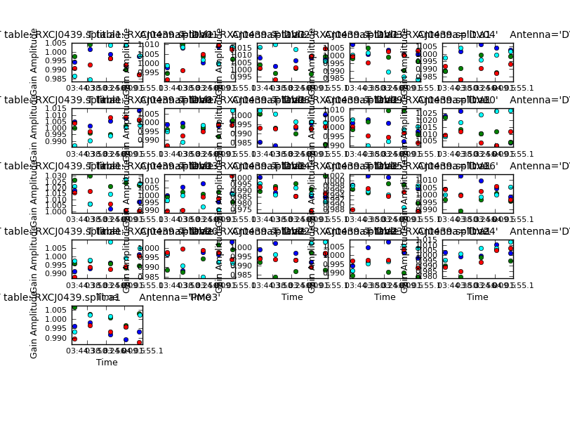
In each round of self-calibration, change at least one of the solution type ('p' or 'a'), solint or other averaging and the model. The S/N should improve for each round. The image peak flux may increase after the first phase corrections, but after that it should only change by a small fraction if at all, and not decrease. This is equivalent to saying that the amplitude solutions should be within a few tens percent of 1. In particular, very low values mean very low data, probably due to decorrelation, which will add noise - either change the calibration strategy or flag the offending data.
Applying solutions: There should be only a few failed solutions (say, <10%). If more, check whether you have used a bad model, applied the wrong gain table, or used an inappropriate solution interval. In some cases there might be much really bad data, but not for this target. If you are not sure whether a few solutions failed due to bad data or an imperfect model, use applymode='calonly'; otherwise use 'calflag' which will flag the data associated with failed solutions. Whatever calibration tables (if any) are applied in gaincal must also be applied in applycal along with the table which you have generated.
Phase (left) and amp (right) solutions, all within acceptable ranges.
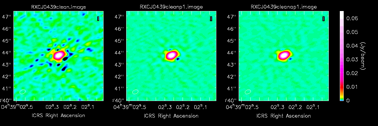
Images left to right: Before any self-calibration, dominated by anti-symmetric errors; after phase self-cal, errors much smaller and more symmetric; a modest improvement after amp self-cal.
You might decide to do more rounds of self-calibration, maybe with a shorter phase solint. Make sure that you always insert the best available model into the MS with ft.
Here, the line is quite weak and is in absorption, but if you had a very strong emission line with better S/N than the continuum, this could be used for self-calibration, applying the solutions to the continuum.